Normality is one assumption that you will typically encounter in statistical methods that you will employ. A lot of the tests that were created have an underlying assumption that your data is normal.

A large number of parametric tests assume normality of data. Ordinary least squares regression assumes it for its error terms, too. You can diagnose your data for normality in the statistical programming language R. The companion software, RStudio, will make everything easier for you. The good news is, you can do it for free.

If you are an Ubuntu user, here’s how to install R.

Requirements

To perform the normality tests, you should have installed the following beforehand:

• R (at least version 3.6.0)
• RStudio (download it here)
• R’s olsrr package

Performing the Tests

For the purpose of this tutorial, let’s generate a data set to perform the tests on by executing the following code:

> data <- rnorm(100)

This code will generate 100 random numbers that follow a standard normal distribution. Our data may differ with one another, but we will expect them to be normal.

Now, there are two ways to diagnose your data for normality:

• Through visual inspection,
• Through statistical tests.

You can’t just use one or the other. You have to use both methods to diagnose your data.

Visual Inspection

The first method is by visual inspection. The way to do this is to generate normal quantile-quantile plots (Q-Q plots). Q-Q  plots will compare your data with the theoretical normal behavior. If your data falls in a straight diagonal line, then your data is most likely normal.

We can do this by using R’s  qqnorm( ) function:

qqnorm(data)

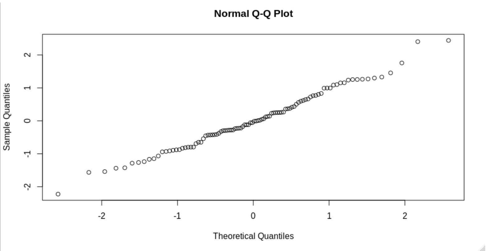
Running this line of code will yield a plot similar to this:

Now we see that the data points follow an approximately straight line. You wouldn’t suspect it to be not normal.

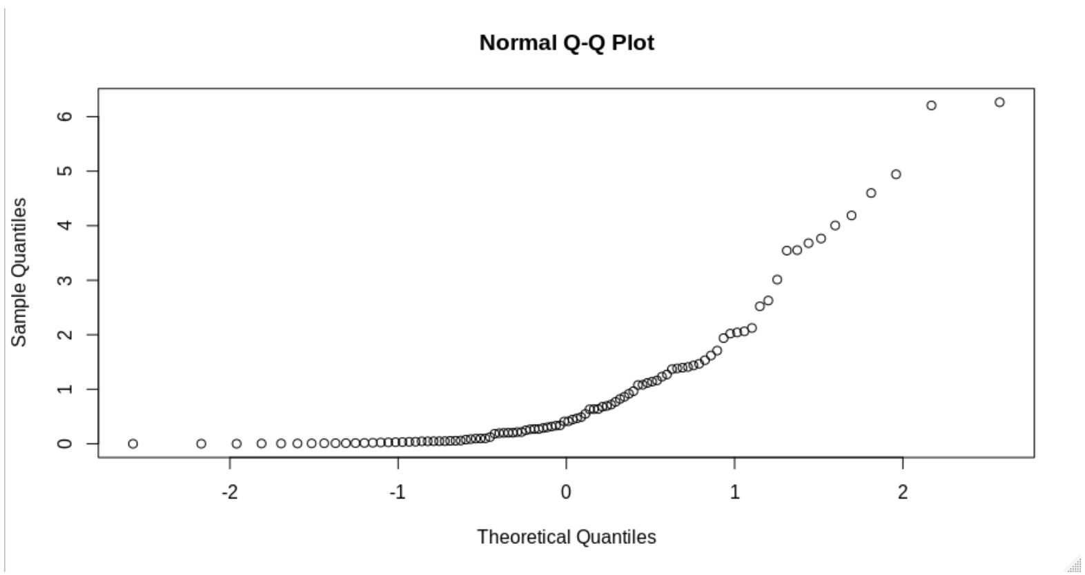
A non-normal data would look like something like this:

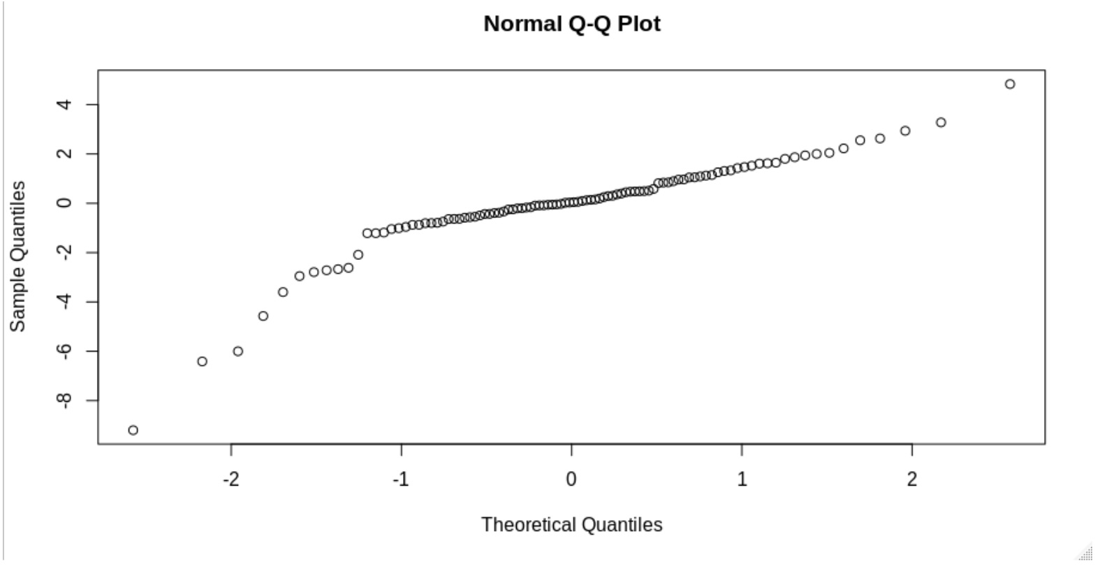
Or something like this:

Now that we have concluded that our data is most likely normal, we can further confirm this by running some statistical tests.

Statistical Tests

There are a lots of normality tests. R’s olsrr package will let you perform several normality tests at once. If you haven’t installed it yet, do so by executing the following line:

> install.packages("olsrr")

After this, load the package using the next line:

require(olsrr)

Now that you have the olsrr package loaded, you’re ready to go. Execute the following line to conduct the normality tests:

> ols_test_normality(data)

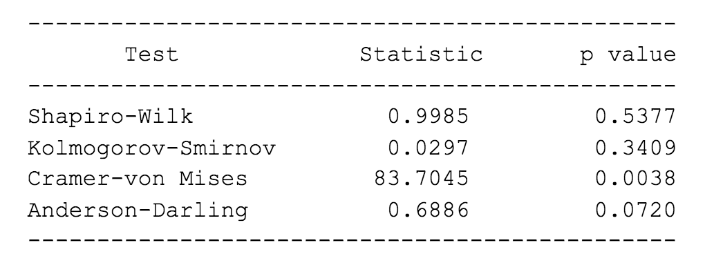
Your output should be something similar:

How would you know if the data is normal according to the tests? The null hypotheses of these tests assume that the data is normal. Let’s assume that the set level of significance is 0.05, the typical level it is set to.

If the p-value is less than the set level of significance, then we are compelled to reject the null hypothesis of normality. Otherwise, we do not reject it.

Three of the tests yielded values that are above 0.05. All of them indicate that we should not reject normality. One test on the other hand, the Cramer-von Mises test, say that the data is not normal.

What happens now?

Most of the time, normality tests agree with one another regarding the normality of data. If not, just like in our case, then check your Q-Q plots in conjunction to the normality tests that you have conducted to see if it is safe to assume normality.

Given our data, despite one test suggesting non-normality, we are compelled to conclude that normality can be safely assumed. Given the visual plots and the number of normality tests which have agreed in terms of their p-values, there is not much doubt.

With this example, we see that statistics does not give perfect outputs. Statistical outputs only serve as guides. We have to use our creativity and the knowledge we have in our field so that we are guided well by the outputs our statistical tools give us.