Machine learning has experienced monumental growth in recent years. We are aware of what can be achieved with machine learning more than ever. The increasing amount of high quality data and advancement in computation have further accelerated the prevalence of machine learning.
There is a wide variety of machine learning algorithms that can be grouped in three main categories:
- Supervised learning algorithms model the relationship between features (independent variables) and a label (target) given a set of observations. Then the model is used to predict the label of new observations using the features. Depending on the characteristics of target variable, it can be a classification (discrete target variable) or a regression (continuous target variable) task.
- Unsupervised learning algorithms try to find the structure in unlabeled data.
- Reinforcement learning works based on an action-reward principle. An agent learns to reach a goal by iteratively calculating the reward of its actions.
In this article, I will briefly explain 15 popular machine learning algorithms in the supervised and unsupervised categories.
The algoritms we will cover are:
- Linear regression
- Logistic regression
- Support vector machine
- Naive bayes
- K-nearest neighbors
- Decision tree
- Random forest
- Gradient boosted decision trees
- LightGBM
- CatBoost
- XGBoost
- K-means clustering
- Hierarchical clustering
- DBSCAN clustering
- Principal component analysis
1. Linear regression
Linear regression is a supervised learning algorithm that models the relationship between a continuous target variable and one or more independent variables by fitting a linear equation to the data.
For a linear regression to be a good choice, there needs to be a linear relation between independent variable(s) and target variable. We can use scatter plots or residual plots to check the linearity.
A linear regression model tries to fit a regression line to the data points that best represents the relations or correlations. The most common technique is ordinary-least squares (OLE) which finds the best regression line by minimizing the sum of squares of the distance between data points and the regression line.
The following plot shows a linear regression line that tried to model the relationship between speed and dist variables based on the given data points.


2. Logistic regression
Logistic regression is a supervised learning algorithm which is mostly preferred for binary classification tasks such as churn prediction, spam email detection, and ad click predictions.
The core part of logistic regression is the logistic (i.e. sigmoid) function. It takes in any real valued number and maps it to a value between 0 and 1.


Logistic regression model takes a linear equation as input to the sigmoid function and uses log odds to perform a binary classification task.
Logistic regression returns probability values. Below is a typical logistic regression curve.

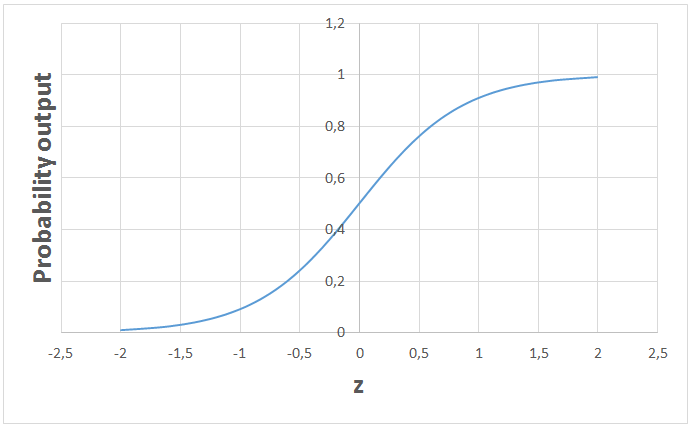
We can use the probability values or convert them to labels (e.g. 1 and 0). For instance, if the probability is greater than 50%, the prediction is positive class (1). Otherwise, the prediction is negative class (0).
The value that serves as a threshold between positive and negative class is problem-dependent. We can adjust the threshold that separates the positive class from the negative class. If it is set as 70%, only the observations with a predicted probability of more than 70% will be classified as positive class.
3. Support vector machine (SVM)
SVM is a supervised learning algorithm that is mostly used for classification tasks.
SVM generates a decision boundary to separate the classes. Before creating the decision boundary, each observation (or row) is plotted in n-dimensional space (n is the number of features). For instance, if we use “length” and “width” to classify different “cells”, observations are plotted in a 2-dimensional space and decision boundary is a line.
Support vectors are the closest data points to the decision boundary. Decision boundary is drawn in a way that the distance to support vectors are maximized.


If the decision boundary is too close to a support vector, it will be highly sensitive to noises and not generalize well. Even very small changes in features may change the prediction.

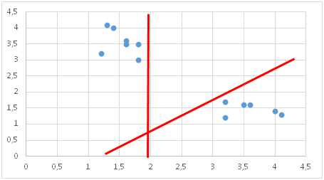
If the data points are not linearly separable, SVM uses a kernel trick which measures the similarity (or closeness) of data points in a higher dimensional space. SVM with a kernel does not actually transform the data points into a higher dimensional space which would not be efficient. It only measures the similarity in a higher dimensional space.
A standard SVM tries to separate all data points in different classes and does not allow any points to be misclassified. This results in an overfit model or, in some cases, a decision boundary cannot be found with a standard SVM.
A better alternative is the soft margin SVM which tries to solve an optimization problem with following goals:
- Increase the distance of decision boundary to classes (or support vectors)
- Maximize the number of points that are correctly classified in training set
The algorithm allows for misclassification of some data points in order to determine a more robust and generalized decision boundary.
There is a trade-off between the two objectives listed above. This trade-off is controlled by C parameter which adds a penalty for each misclassified data point. If c is small, penalty for misclassified points is low so a decision boundary with a large margin is chosen at the expense of a greater number of misclassifications. If c is large, SVM tries to minimize the number of misclassified examples due to high penalty which results in a decision boundary with a smaller margin. Penalty is not same for all misclassified examples. It is directly proportional to the distance to decision boundary.
4. Naive Bayes
Naive Bayes is a supervised learning algorithm used for classification tasks.
Naive Bayes assumes that features are independent of each other and there is no correlation between features. However, this is not the case in real life. This naive assumption of features being uncorrelated is the reason why this algorithm is called “naive”.
As the name suggests, the core element of this algorithm is the Bayes’ theorem.


p(A|B): Probability of event A given event B has already occurred
p(B|A): Probability of event B given event A has already occuured
p(A): Probability of event A
p(B): Probability of event B
Naive Bayes calculates the probability of a class given a set of feature values (i.e. p(yi | x1, x2 , … , xn)). Under the assumption of features being independent, we can use this probability and the Bayes’ Theorem to achieve:


The algorithm converts a complex conditional probability into the product of much simpler conditional probabilities.
The assumption that all features are independent makes naive bayes algorithm very fast compared to complicated algorithms. In some cases, speed is preferred over higher accuracy. On the other hand, the same assumption makes naive bayes algorithm less accurate than complicated algorithms. Speed comes at a cost!
5. K-nearest neighbors
K-nearest neighbors (kNN) is a supervised learning algorithm that can be used to solve both classification and regression tasks. The main idea is that the value or class of a data point is determined by the data points around it.
kNN classifier determines the class of a data point by majority voting principle. For instance, if k is set to 5, the classes of 5 closest points are checked. Prediction is done according to the majority class. Similarly, kNN regression takes the mean value of 5 closest points.
The biggest challenge of kNN is to determine the optimal value for k. Very small k values tend to result in overfitting because the model is too specific to the training set and not generalized well. On the other hand, models with very large k values are not good predictors on both train and test sets. They tend to be underfitting.
kNN is simple and easy to interpret. It does not make any assumption so it can be implemented in non-linear tasks. kNN becomes very slow as the number of data points increases because the model needs to store all data points. Thus, it is also not memory efficient. Another downside of kNN is that it is sensitive to outliers.
6. Decision tree
Decision tree is a supervised learning algorithm. It partitions the data points (i.e. rows) by iteratively asking questions.

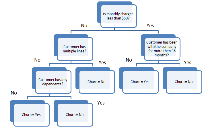
The splits are not determined randomly. The ones that result in the highest information gain are selected. Splits that increase the purity of nodes are more informative.
The purity of a node is inversely proportional to the distribution of different classes in that node. The questions to ask are chosen in a way that increases purity or decrease impurity.
The algorithm keeps asking questions until all the nodes are pure. Pure nodes only contains observations of one specific class. However, this would be a too specific model and would not generalize well. Decision tree algorithm can easily be overfit if we do not set a limit on the depth. The depth of a tree is controlled by the max_depth parameter.
Decision tree algorithm usually does not require to normalize or scale features. It is also suitable to work on a mixture of feature data types (continuous, categorical, binary).
7. Random forest
Random forest is a supervised learning algorithm. A random forest is an ensemble of decision trees combined with a technique called bagging.
In bagging, decision trees are used as parallel estimators. Having many decision trees combined in parallel greatly reduces the risk of overfitting and results in a much more accurate model.
The success of a random forest highly depends on using uncorrelated decision trees. If we use same or very similar trees, the overall result will not be much different than the result of a single decision tree. Random forests achieve to have uncorrelated decision trees by bootstrapping and feature randomness.
Bootsrapping is randomly selecting samples from training data with replacement. They are called bootstrap samples.
Feature randomness is achieved by selecting features randomly for each decision tree in a random forest. The number of features used for each tree in a random forest can be controlled with max_features parameter.


Random forest is a highly accurate model on many different problems and does not require normalization or scaling.
8. Gradient boosted decision trees (GBDT)
GBDT is a supervised learning algorithm that is built by combining decision trees with a technique called boosting. Thus, GBDT is also an ensemble method.
Boosting means combining a learning algorithm in series to achieve a strong learner from many sequentially connected weak learners.
Each tree attempts to minimize the errors of previous tree. Trees in boosting are weak learners but adding many trees in series and each focusing on the errors from previous one make boosting a highly efficient and accurate model. Unlike bagging, boosting does not involve bootstrap sampling. Every time a new tree is added, it fits on a modified version of initial dataset.

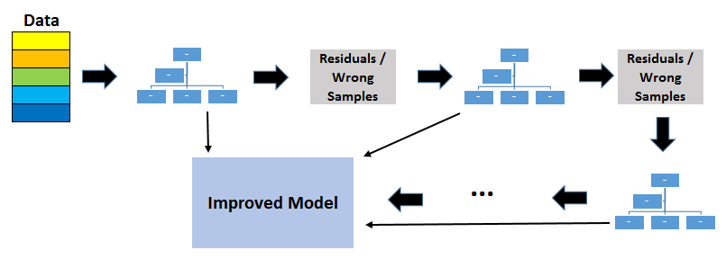
Since trees are added sequentially, boosting algorithms learn slowly. In statistical learning, models that learn slowly perform better.
Learning rate and n_estimators are two critical hyperparameters for GBDT. Learning rate, denoted as α, simply means how fast the model learns. Each new tree modifies the overall model. The magnitude of the modification is controlled by learning rate. N_estimator is the number of trees used in the model. If the learning rate is low, we need more trees to train the model. However, we need to be very careful at selecting the number of trees. It creates a high risk of overfitting to use too many trees.
GBDT is very efficient on both classification and regression tasks and provides more accurate predictions compared to random forests. It can handle mixed type of features and no pre-processing is needed. GBDT requires careful tuning of hyperparameters in order to prevent the model from overfitting.
GBDT algorithm is so powerful that there are many upgraded versions of it have been implemented such as XGBOOST, LightGBM, CatBoost.
9. LightGBM
LightGBM, created by researchers at Microsoft, is an implementation of gradient boosted decision trees.
Decision trees are built by splitting observations (i.e. data instances) based on feature values. This is how a decision tree “learns”. The algorithm looks for the best split which results in the highest information gain.
Finding the best split turns out to be the most time-consuming part of the learning process of decision trees. As the size of data increases, this becomes a bottleneck. LightGBM is aimed to solve this efficiency problem, especially with large datasets.
To overcome this issue, LightGBM uses two techniques:
- GOSS (Gradient One-Side Sampling)
- EFB (Exclusive Feature Bundling)
I will not go in detail but here is a more detailed article that I wrote to explain how LightGBM works.
10. CatBoost
LightGBM, created by researchers at Yandex, is another implementation of gradient boosted decision trees.
Since we have already covered GBDT, I will only mention the characteristic features of CatBoost.
CatBoost implements a specific version of boosting which is called ordered boosting. It provides a better approach for handling overfitting. CatBoost also has a great performance at handling categorical features. Another distinctive feature is using symmetric trees.
Official documentation and this tutorial provides a comprehensive guide for understanding and using the CatBoost algorithm.
11. XGBoost
XGBoost is another implementation of GBDT. It was so powerful that it dominated some major kaggle competitions. The goal of XGboost, as stated in its documentation, “is to push the extreme of the computation limits of machines to provide a scalable, portable and accurate library”.
One common feature of XGBoost, LightGBM, and CatBoost is that they require careful tuning of hyperparameters. The performance of models highly depend on selecting the optimal hyperparameter values.
For instance, below is a typical list of hyperparameters for a XGBoost model to solve a multi-class classification task.
params_xgb = {
'boosting_type': 'dart',
'objective':'multi:softmax',
'num_class':9,
'max_depth':7,
'min_child_weight':20,
'gamma':1,
'subsample':0.8,
'colsample_bytree':0.7,
'tree_method':'hist',
'eval_metric':'mlogloss',
'eta':0.04,
'alpha': 1,
'verbose': 2
}
- Max_depth: The maximum depth of a tree.
- Min_child_weight: The minimum sum of instance weight needed in a child. Keeping it high prevents the child from being too specific and thus helps to avoid overfitting.
- Gamma: Minimum loss reduction required to make a further partition on a leaf node of the tree. Again, the larger the game, the less likely the model will overfit.
- Subsample: The ratio of rows that are randomly selected prior to growing trees. Subsample can also be used to avoid overfitting.
- Eta: The learning rate. Keeping it high makes the model learn fast but increases the chance of overfitting at the same time.
- Alpha: L1 regularization term.
The entire list of hyperparameters of XGBoost can be found here.
12. K-means clustering
K-means clustering is an unsupervised learning algorithm. It aims to partition data into k clusters in a way that data points in the same cluster are similar and data points in the different clusters are farther apart. Thus, it is a partition-based clustering technique. Similarity of two points is determined by the distance between them.
It is important to note that this is different than classification where we have attached labels for the data points in the training set. In clustering, the data points do not have labels. The algorithm is expected to find the structure within the data to group data points into clusters.
K-means clustering tries to minimize distances within a cluster and maximize the distance between different clusters.
The biggest challenge of k-means clustering is to determine the optimal value for the number of cluster. The algorithm cannot determine the number of clusters so we need to specify it.

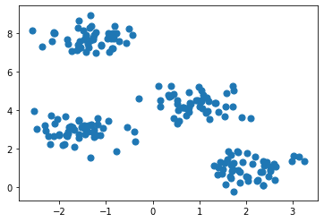

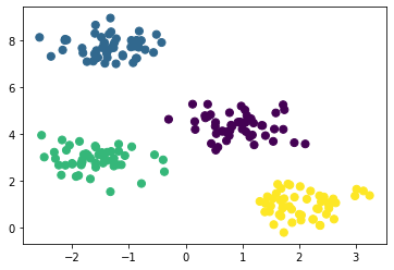
K-Means clustering is relatively fast and easy to interpret. It is also able to choose the positions of initial centroids (center of cluster) in a smart way that speeds up the convergence.
13. Hierarchical clustering
Hierarchical clustering is an unsupervised learning algorithm. It creates a tree of clusters by iteratively grouping or separating data points. There are two types of hierarchical clustering:
- Agglomerative clustering
- Divisive clustering

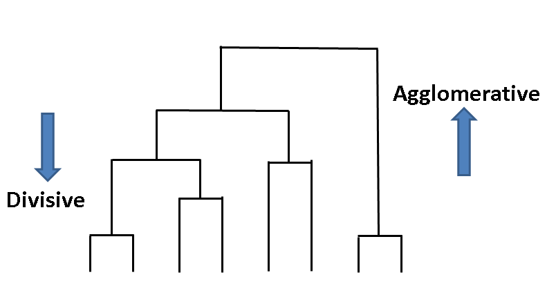
Agglomerative is the most commonly used approach. Each data point is assumed to be a separate cluster at first. Then the similar clusters are iteratively combined.
One of the advantages of hierarchical clustering is that we do not have to specify the number of clusters beforehand. However, it is not wise to combine all data points into one cluster. We should stop combining clusters at some point.
Hierarchical clustering always generates the same clusters. K-means clustering may result in different clusters depending on how the centroids (center of cluster) are initiated. However, it is a slower algorithm compared to k-means. Hierarchical clustering takes long time to run especially for large datasets.
14. DBSCAN clustering
Partition-based and hierarchical clustering techniques are highly efficient with normal shaped clusters. However, when it comes to arbitrary shaped clusters or detecting outliers, density-based techniques are more efficient.
DBSCAN stands for density-based spatial clustering of applications with noise. It is able to find arbitrary shaped clusters and clusters with noise (i.e. outliers).

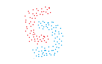
The main idea behind DBSCAN is that a point belongs to a cluster if it is close to many points from that cluster.
There are two key parameters of DBSCAN:
- eps: The distance that specifies the neighborhoods. Two points are considered to be neighbors if the distance between them are less than or equal to eps.
- minPts: Minimum number of data points to define a cluster.
Based on these two parameters, points are classified as core point, border point, or outlier:
- Core point: A point is a core point if there are at least minPts number of points (including the point itself) in its surrounding area with radius eps.
- Border point: A point is a border point if it is reachable from a core point and there are less than minPts number of points within its surrounding area.
- Outlier: A point is an outlier if it is not a core point and not reachable from any core points.
DBSCAN does not require to specify number of clusters beforehand. It is robust to outliers and able to detect the outliers.
In some cases, determining an appropriate distance of neighborhood (eps) is not easy and it requires domain knowledge.
15. Principal component analysis (PCA)
PCA is a dimensionality reduction algorithm which basically derives new features from the existing ones with keeping as much information as possible. PCA is an unsupervised learning algorithm but it is also widely used as a preprocessing step for supervised learning algorithms.
PCA derives new features by finding the relations among features within a dataset.
PCA is a linear dimensionality reduction algorithm. There are also non-linear methods available.
The aim of PCA is to explain the variance within the original dataset as much as possible by using less features (or columns). The new derived features are called principal components. The order of principal components is determined according to the fraction of variance of original dataset they explain.
The principal components are linear combinations of the features of original dataset.
The advantage of PCA is that a significant amount of variance of the original dataset is retained using much smaller number of features than the original dataset. Principal components are ordered according to the amount of variance they explain.
Conclusion
We have covered the most commonly used machine learning algorithms used in the field of data science. I tried to provide a decent introduction for each model. You need to go a little deeper and also practice in order to master each algorithm.

